Asymptotic Complexity Explained
“Simplicity is a great virtue but it requires hard work to achieve it and education to appreciate it. And to make matters worse: complexity sells better.”
– Edsger W. Dijkstra
Ever wondered what asymptotic complexity or Big-\(\mathcal{O}\) notation are or what they mean mathematically? This post will explain asymptotic complexity without handwaving as much of the math. This post is meant for someone who has heard of Big-O but doesn’t know exactly what it means. If you want an even deeper more rigorious look at this subject, I recommend reading chapter 3 of CLRS.
Let’s start with computational complexity. The computational complexity of an algorithm is a measure of the resources the algorithm needs to run. These resources are typically significant considerations to the real world application of the algorithm such as the running time and space in memory used by the algorithm.
We can think of the time complexity of an algorithm being a function \( T(n) \) where \(n\) is the size of the input to the algorithm. The asymptotic complexity of \( T(n) \) is a way we describe the behavior of the function’s complexity for larger and larger input sizes (how it behaves closer to the asymptote).
To describe asymptotic complexity, we use Big-\(\mathcal{O}\) notation which allows us to talk precisely about the limiting behavior of a function. This “limiting behavior” is how the function behaves as \(n\) approaches \( \infty \).
I’ll quickly describe Big-\(\mathcal{O}\), Big-\(\Omega\), and Big-\(\Theta\) but there are lots of other notations that exist like little-o or little-\(\omega\) which is out of the scope of this post.
Big-\(\mathcal{O}\)
We use Big-\(\mathcal{O}\) to denote an asymptotic upper bound on a function i.e. a bound on the worst case. “It can’t get worse than this.”
To better understand what this means, below is the formal definition of Big-\(\mathcal{O}\) for a given function \(g(n)\).
\[ \mathcal{O}(g(n)) = \{f(n) \mid \exists \ c, n_0 \in \mathbb{R^+} \ \mathrm{s.t.} \ 0 \leq f(n) \leq cg(n) \ \forall n \geq n_0 \} \]
To put that into words, \(\mathcal{O}(g(n))\) is the set of all functions for which you can always find a positive integer \(c\) such that \(cg(n)\) is always greater than or equal to that function starting at a sufficiently large value \(n_0\).
btw just as a quick aside, we always assume that \(T(n)\) is a function from positive integers to nonnegative real numbers. We also assume that \(T(n)\) is asymptotic positive, meaning that for a sufficiently large input, the output of \(T(n)\) will be positive.
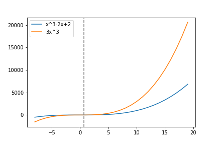
This is easier to see visually and through example. Take the above graph. The blue line represents the running time function \(h(n) = n^3-2n+2\). The function \(h(n)\) is in the set \(\mathcal{O}(n^3)\) because if we pick \(c=3\) and start at \(n_0 \approx 0.68233\) (the gray line) then \( cn^3 \geq h(n) \) for all \( n \geq n_0 \) which implies that \( h(n) \in \mathcal{O}(n^3) \) by the definition of Big-\(\mathcal{O}\).
Another quick aside, computer scientists often will write the last statement as \( h(n)=\mathcal{O}(n^3)\). This is an abuse of notation that I will use as well and that you will see frequently, but just remember that it is an abuse of notation and that the equal sign as it is used here is asymmetric (i.e. \( \mathcal{O}(n^3) \ne h(n)\)). It is useful to read the statement as just “\(h(n)\) is in \(\mathcal{O}(n^3)\).”
Big-\(\Omega\)
Big-\(\Omega\) is the lower bound counterpart to Big-\(\mathcal{O}\). It is a bound on the best case of an algorithm. Normally, in computer science, we are more worried about the worst case performance of an algorithm but in some cases, lower bound analysis is useful.
When is knowing a lower bound useful? An example would be knowing that the sorting problem using the comparison model (sorting via comparing two numbers) is bounded by \( \Omega(n \lg n) \). This means that it isn’t possible to create an algorithm that sorts a sequence of numbers via comparisons faster than \( \Omega(n \lg n) \).
 Big-\(\Omega\) says “it can’t be better than this.”
The formal definition of \(\Omega\) is the same as \(\mathcal{O}\) except with the order of \( cg(n) \) and \( f(n)\) switched.
\[ \Omega(g(n)) = \{f(n) \mid \exists \ c, n_0 \in \mathbb{R^+} \ \mathrm{s.t.} \ 0 \leq cg(n) \leq f(n) \ \forall n \geq n_0 \} \]
Big-\(\Theta\)
Big-\(\Theta\) is an asymptotically tight bound on a function. You can think of \(\Theta\) is the intersection between \(\mathcal{O}\) and \(\Omega\). Big-\(\Theta\) is both a lower bound and an upper bound.
\[ \Theta(g(n)) = \mathcal{O}(g(n)) \cap \Omega(g(n)) \]
Also, the following is true,
\[h(n) \in \Theta(g(n)) \iff h(n) \in \mathcal{O}(g(n)) \ \mathrm{and} \ h(n) \in \Omega(g(n)) \mathrm{.} \]
Finally, here is the definition in set builder notation and as you can probably guess, is a mix of the definitions of \(\mathcal{O}\) and \(\Omega\).
\[ \Theta(g(n)) = \{f(n) \mid \exists \ c_1, c_2, n_0 \in \mathbb{R^+} \ \mathrm{s.t.} \ 0 \leq c_1g(n) \leq f(n) \leq c_2g(n) \ \forall n \geq n_0 \} \]
The definition is essentially a “sandwiching” of \(f(n)\) between \( c_1g(n)\) and \( c_2g(n)\).
Conclusion
Asymptotic complexity is an invaluable tool for computer scientists to describe and compare algorithms in a hardware-agnostic manner and I strongly believe that understanding the math behind it helps with understanding the concept intuitively. I hope this post helped explain the math behind asymptotic complexity in a clear way!
– pry